Matyas Function
Mathematical Definition
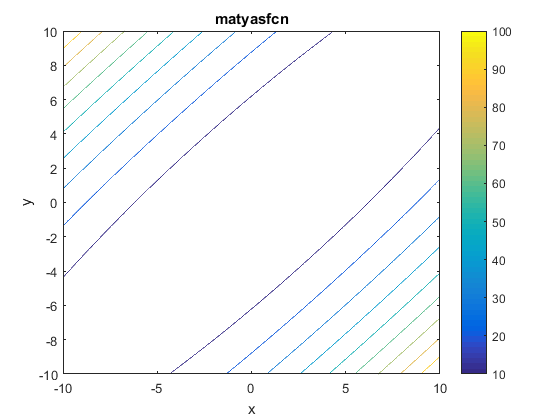
\[f(x, y)=0.26(x^2+y^2) -0.48xy\]Plots
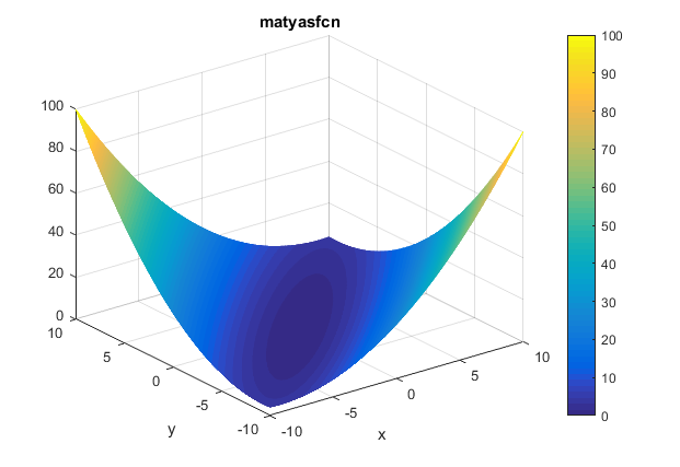
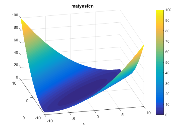
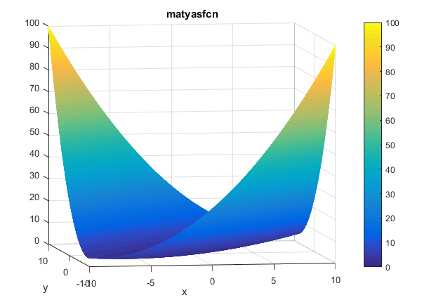
The contour of the function is as presented below:
Description and Features
- The function is continuous.
- The function is convex.
- The function is defined on 2-dimensional space.
- The function is unimodal.
- The function is differentiable.
- The function is non-separable.
- The function is .
Input Domain
The function can be defined on any input domain but it is usually evaluated on $x \in [-10, 10]$ and $y \in [-10, 10]$ .
Global Minima
The function has one global minimum $f(\textbf{x}^{\ast})=0$ at $\textbf{x}^{\ast} = (0, 0)$.
Implementation
Python
For Python, the function is implemented in the benchmarkfcns package, which can be installed from command line with pip install benchmarkfcns.
from benchmarkfcns import matyas

print(matyas([[0, 0],
              [1, 1]]))
MATLAB
An implementation of the Matyas Function with MATLAB is provided below.
% Computes the value of the Matyas benchmark function.
% SCORES = MATYASFCN(X) computes the value of the Matyas function at
% point X. MATYASFCN accepts a matrix of size M-by-2 and returns a
% vetor SCORES of size M-by-1 in which each row contains the function value
% for the corresponding row of X.
% For more information please visit:
% https://en.wikipedia.org/wiki/Test_functions_for_optimization
%
% Author: Mazhar Ansari Ardeh
% Please forward any comments or bug reports to mazhar.ansari.ardeh at
% Google's e-mail service or feel free to kindly modify the repository.
function scores = matyasfcn(x)
    n = size(x, 2);
    assert(n == 2, 'Matyas''s function is only defined on a 2D space.')
    X = x(:, 1);
    Y = x(:, 2);

    scores = 0.26 * (X .^ 2 + Y.^2) - 0.48 * X .* Y;
end
The function can be represented in Latex as follows:
f(x, y)=0.26(x^2+y^2) -0.48xyReferences:
- http://www.sfu.ca/~ssurjano/matya.html
- https://en.wikipedia.org/wiki/Test_functions_for_optimization
- Momin Jamil and Xin-She Yang, A literature survey of benchmark functions for global optimization problems, Int. Journal of Mathematical Modelling and Numerical Optimisation}, Vol. 4, No. 2, pp. 150–194 (2013), arXiv:1308.4008